[prev] [up] [next]

The ST/X Constraint Solver

Contents

Introduction

The ST/X Constraint Solver package provides classes to represent constraint variables, expressions, domains and a backtracking solver, with configurable and extendable variable and domain selection stategies.

Problem definition is straight forward, using the Smalltalk language itself. Due to the expressiveness of the smalltalk language, no DSL is needed; in fact, problem definitions in Smalltalk look almost similar (and often even easier to write and understand) than definitions in other CSP systems, even some with specific constraint definition languages.

The ST/X constraint solver can be used to solve puzzles, crosswords, sodoku, scheduling tasks and electronic design problems.

Feature List

Domain Types: Constraint Expressions: Domain partitioning/enumeration strategies: Variable selection strategies:

Gentle Introduction

A First Example

For motivation, let's start with a well-known, very simple example, the SEND-MORE-MONEY puzzle. This puzzle's goal is to find the digit-values for the variables S,E,N,D,M,O,R and Y, such that:

      SEND
   +  MORE
   -------
   = MONEY

is a valid arithmetic expression.

Here is the complete code to solve this puzzle; the explanation follows right below:
    |result|

    result :=
	Solver anySolutionFor:[
	    |S E N D M O R Y|

	    S := (1 %% 9) name:'S'.
	    E := (0 %% 9) name:'E'.
	    N := (0 %% 9) name:'N'.
	    D := (0 %% 9) name:'D'.
	    M := (1 %% 9) name:'M'.
	    O := (0 %% 9) name:'O'.
	    R := (0 %% 9) name:'R'.
	    Y := (0 %% 9) name:'Y'.

	    Solver allDistinct:{ S . E . N . D . M . O . R . Y }.

			     ((S*1000) + (E*100) + (N*10) + D)
	      +              ((M*1000) + (O*100) + (R*10) + E)
	      =: ((M*10000) + (O*1000) + (N*100) + (E*10) + Y).
	].

    Transcript showCR:('result = %1' bindWith:result).
    Transcript showCR:''.

    Transcript showCR:('   %(S)%(E)%(N)%(D)' bindWithArguments:result).
    Transcript showCR:('+  %(M)%(O)%(R)%(E)' bindWithArguments:result).
    Transcript showCR:('-------').
    Transcript showCR:('= %(M)%(O)%(N)%(E)%(Y)' bindWithArguments:result).
The expression "Solver anySolutionFor:[...]" asks the solver to provide a solution for the problem which is specified by the block argument. Inside the block, we first declare the problem variables as FD (Finite-Domain) variables, being a digit in the range 0..9 (except for M and S, which cannot be '0', as they are used in the high decimal position):
    |S E N D M O R Y|

    S := (1 %% 9) name:'S'.
    E := (0 %% 9) name:'E'.
    N := (0 %% 9) name:'N'.
    D := (0 %% 9) name:'D'.
    M := (1 %% 9) name:'M'.
    O := (0 %% 9) name:'O'.
    R := (0 %% 9) name:'R'.
    Y := (0 %% 9) name:'Y'.
the "min %% max"-construct is of course a message-send to min (a Number), and a shortcut for "FDVariable integer:(min to: max)", which itself is a shortcut for "FDVariable new domain:(IntegerDomain min:min max:max)". All of them create a new FD-variable with an integer domain, limiting their possible values to 0..9 (1..9 for the two exceptions S and M).

Giving each variable a name is not required by the solver; however, the solution's print-string looks nicer if we do so. Also the formatted-string printing at the end requires named values in the solution vector (without proper names, individual variables from the solution vector must be accessed via a numeric index).

The next expression:
    Solver allDistinct:{ S . E . N . D . M . O . R . Y }.
states that all the variables take on different values. Without this declaration, the solver might find "(S=9 E=0 N=0 D=0 M=1 O=0 R=0 Y=0)" as a solution.

Next, we declare that the decimal value of SEND and MORE results in MONEY:
		   ((S*1000) + (E*100) + (N*10) + D)
    +              ((M*1000) + (O*100) + (R*10) + E)
    =: ((M*10000) + (O*1000) + (N*100) + (E*10) + Y).
Notice that we have to construct the two addends by scaling the digits according to their decimal position. Also notice the special "=:" operator (colon on the right), which is called the "unification" operator; it enforces the two constraint expressions to be unified to the same value The "(a =: b)" expression can be considered as a shortcut for "(a = b) =: true", i.e. state that the proposition "(a = b)" must be true in the solution).

Also notice, that due to the precedence rules of the Smalltalk language, both sides of the unification operator have to be parenthized (Smalltalk language-wise, "=:" is a binary operator with the same precedence as the "+" or "-" messages)

This specification-block is given to the solver, and asked to return any solution. The resturned result vector is:
Solution(S->9 E->5 N->6 D->7 M->1 O->0 R->8 Y->2)
As we get the result as an ordered dictionary, which maps both variable names and numeric indices to solution-values, and thanks to giving them variables a name, we can pretty-print the solution easily with:
    Transcript showCR:('   %(S)%(E)%(N)%(D)' bindWithArguments:result).
    Transcript showCR:('+  %(M)%(O)%(R)%(E)' bindWithArguments:result).
    Transcript showCR:('-------').
    Transcript showCR:('= %(M)%(O)%(N)%(E)%(Y)' bindWithArguments:result).
which prints:
   9567
+  1085
-------
= 10652

Finite Domain Variables

When specifying a problem, a set of FD-expressions is created. FD expressions consist of a variable or arithmetic-expression, a domain, which limits the set of possible values it can take. Hidden to our eyes is the set of propagators, which notify other constraint expressions whenever this domain changes. Whenever new information arrives (for example, during the declaration phase), or when the solver tries to set a variable's value, information about these domain changes is passed around via the propagators, and other domains are adjusted as required. The goal of those propagators is to delimit the domains of each variable as much as possible, in order to reduce the number of possible value-combinations which gave to be tried by the solver.

For example, if we define two variables A,B each with possible values from [0..5] and a sum of them with:
    |A B sum|

    A := 0 %% 5.
    B := 0 %% 5.
    sum := A + B.
each FD-expression already has an idea of what its possible domain is. The domain is shown in the printString, but there are also accessors (domain and domain:). The printStrings of A, B and sum are:
    ?expr?:(0..5)
    ?expr?:(0..5)
    (?expr?)+(?expr?):(0..10)
For A, B, this was obvious, as we had specified it before. However, for sum, the domain was computed automatically.

We get nicer printStrings, if we give each a name:
    |A B sum|

    A := 0 %% 5.
    B := 0 %% 5.
    sum := A + B.

    A name:'A'.
    B name:'B'.
    sum name:'sum'.

    Transcript showCR:A.
    Transcript showCR:B.
    Transcript showCR:sum.
we get:
A:(0..5)
B:(0..5)
sum "(A)+(B)":(0..10)
Now, lets assume, that we know that the result from multiplying A and B is positive:
    A * B >: 0.
looking now at the variables, we get:
    A:(1..5)
    B:(1..5)
    sum "(A)+(B)":(2..10)
i.e. the constraint propagators found out themself, that A and B cannot be 0, and that the sum must therefore be 2 or larger.

We might even know that the sum has certain qualities:
    sum <=: 5.
which further reduces the domains of A and B:
    A:(1..4)
    B:(1..4)
    sum "(A)+(B)":(2..5)

Searching a Valid Combination

Once we have defined the set of constraints, the solver starts to systematically generate and validate a set of possible value combinations. In the above example, a naïve algorithm might try (1..4)x(1..4) = 16 combinations. However, due to the propagation of changes into the domains, every tried value-choice immediately affects the domains of all dependent variables. For example, if the solver tries a value of 3 as a possible value for A, the domain for B changes to (1..2). I.e. the values 0, 3, 4 and 5 are NEVER even considered in combination with A=3.
Effectively, in the above example, the tried combinations will only be:
    A = 1, B = 1
    A = 1, B = 2
    A = 1, B = 3
    A = 1, B = 4

    A = 2, B = 1
    A = 2, B = 2
    A = 2, B = 3

    A = 3, B = 1
    A = 3, B = 2

    A = 4, (B automatically constraint to 1)

Pruning the Solver's Search Tree

The domain information is used by the solver to prune the searchtree, when it tries all possible variable value combinations. The following example demonstates this::

Without additional domain information, all possible combinations are tried:
    Solver
	allSolutionsFor:[
	    |x y z|

	    x := (1 %% 3) name:'x'.
	    y := (1 %% 3) name:'y'.
	    z := (1 %% 3) name:'z'.
	]
	into:[:eachSolution |
	    Transcript showCR:eachSolution.
	].
generates:
    Solution(x->1 y->1 z->1)
    Solution(x->1 y->1 z->2)
    Solution(x->1 y->1 z->3)
    Solution(x->1 y->2 z->1)
    Solution(x->1 y->2 z->2)
    Solution(x->1 y->2 z->3)
    Solution(x->1 y->3 z->1)
    Solution(x->1 y->3 z->2)
    Solution(x->1 y->3 z->3)
    Solution(x->2 y->1 z->1)
    Solution(x->2 y->1 z->2)
    Solution(x->2 y->1 z->3)
    Solution(x->2 y->2 z->1)
    Solution(x->2 y->2 z->2)
    Solution(x->2 y->2 z->3)
    Solution(x->2 y->3 z->1)
    Solution(x->2 y->3 z->2)
    Solution(x->2 y->3 z->3)
    Solution(x->3 y->1 z->1)
    Solution(x->3 y->1 z->2)
    Solution(x->3 y->1 z->3)
    Solution(x->3 y->2 z->1)
    Solution(x->3 y->2 z->2)
    Solution(x->3 y->2 z->3)
    Solution(x->3 y->3 z->1)
    Solution(x->3 y->3 z->2)
    Solution(x->3 y->3 z->3)
with additional constraints, some solutions are not even tried. For example, if we announce that x <= y <= z with:
    Solver
	allSolutionsFor:[
	    |x y z|

	    x := (1 %% 3) name:'x'.
	    y := (1 %% 3) name:'y'.
	    z := (1 %% 3) name:'z'.

	    x <=: y.
	    y <=: z.
	]
	into:[:eachSolution |
	    Transcript showCR:eachSolution.
	].
we get:
    Solution(x->1 y->1 z->1)
    Solution(x->1 y->1 z->2)
    Solution(x->1 y->1 z->3)
    Solution(x->1 y->2 z->2)
    Solution(x->1 y->2 z->3)
    Solution(x->2 y->2 z->2)
    Solution(x->2 y->2 z->3)
    Solution(x->1 y->3 z->3)
    Solution(x->2 y->3 z->3)
    Solution(x->3 y->3 z->3)
If enough information is available, the constraints alone are sufficient to provide a consistent solution. Here is a famous puzzle, asking for how many pigs and hens a farmer has, if the number of legs adds up to 22:
    |pigs hens|

    pigs := (0 %% 7).
    hens := (0 %% 7).

    pigs + hens =: 7.
    (pigs * 4) + (hens * 2) =: 22.

    Transcript showCR:('%1 pigs and %2 hens'
			    bindWith:(pigs value)
			    with:(hens value) ).
With this knowledge, it should be clear, that there are multiple ways to specify a constraint problem, and that the amount of information in form of constraints might affect the overall performance, by possibly reducing the number of value combinations that have to be tried by the solver.
Coming back to the puzzle, an alternative, which makes the additions concrete, could have been:
    |result|

    result :=
	Solver anySolutionFor:[
	    |S E N D M O R Y
	     DE NR EO SM
	     cDE cNR cEO cSM|

	    S := (1 %% 9) name:'S'.
	    E := (0 %% 9) name:'E'.
	    N := (0 %% 9) name:'N'.
	    D := (0 %% 9) name:'D'.
	    M := (1 %% 9) name:'M'.
	    O := (0 %% 9) name:'O'.
	    R := (0 %% 9) name:'R'.
	    Y := (0 %% 9) name:'Y'.

	    Solver allDistinct:{ S . E . N . D . M . O . R . Y }.

	    "/          S    E    N    D
	    "/ +        M    O    R    E
	    "/ -------------------------
	    "/ +  cSM  cEO  cNR  cDE
	    "/ -------------------------
	    "/ =   M    O    N    E    Y

	    DE := (D + E).
	    cDE := (DE // 10).          "/ the carry (tens)
	    Y =: (DE \\ 10).            "/ the digit (ones)
	    "/ Y =: (DE - (cDE * 10)).     "/ another alternative

	    NR := (N + R + cDE).
	    cNR := (NR // 10).          "/ tens
	    E =: (NR \\ 10).            "/ ones

	    EO := (O + E + cNR).
	    cEO := (EO // 10).
	    N =: (EO \\ 10).

	    SM := (S + M + cEO).
	    cSM := (SM // 10).
	    O =: (SM \\ 10).

	    M =: cSM.

	    self halt.
	].

    Transcript showCR:('result = %1' bindWith:result).
    Transcript showCR:''.

    Transcript showCR:('   %(S)%(E)%(N)%(D)' bindWithArguments:result).
    Transcript showCR:('+  %(M)%(O)%(R)%(E)' bindWithArguments:result).
    Transcript showCR:('-------').
    Transcript showCR:('= %(M)%(O)%(N)%(E)%(Y)' bindWithArguments:result).
In the above we deal with the carry from each pair of added digits: DE is the sum of D and E. Y is the ones (DE modulu 10) and cDE is the carry (the tens, (DE divided by 10).

Arriving at the halt at the end of the block, we see that the variables already have much smaller domains:
    var1 . : S:(8..9)
    var2 . : E:(0 | 2..9)
    var3 . : N:(0 | 2..9)
    var4 . : D:(0 | 2..9)
    var5 . : M:1
    var6 . : O:(0 | 2..9)
    var7 . : R:(0 | 2..9)
    var8 . : Y:(0 | 2..9)
    var9 . : (D)+(E):(0..18)
    var10  : (?expr?)+(?expr?):(0..19)
    var11  : (?expr?)+(?expr?):(0..19)
    var12  : (?expr?)+(?expr?):10
    var13  : (?expr?)//(10):(0..1)
    var14  : (?expr?)//(10):(0..1)
    var15  : (?expr?)//(10):(0..1)
    var16  : (?expr?)//(10):1
So, the setup already reduced M's domain to a single value. And also found that S can only take two values. It is obvious, that this reduces the solver's search space.

To get a feeling for the solver's operation, let us trace its set of tried combinations:
    |solver result|

    solver := Solver new.
    solver
	defineProblem:[
	    |S E N D M O R Y
	     DE NR EO SM
	     cDE cNR cEO cSM|

	    S := (1 %% 9) name:'S'.
	    E := (0 %% 9) name:'E'.
	    N := (0 %% 9) name:'N'.
	    D := (0 %% 9) name:'D'.
	    M := (1 %% 9) name:'M'.
	    O := (0 %% 9) name:'O'.
	    R := (0 %% 9) name:'R'.
	    Y := (0 %% 9) name:'Y'.

	    Solver allDistinct:{ S . E . N . D . M . O . R . Y }.

	    "/          S    E    N    D
	    "/ +        M    O    R    E
	    "/ -------------------------
	    "/ +  cSM  cEO  cNR  cDE
	    "/ -------------------------
	    "/ =   M    O    N    E    Y

	    DE := (D + E).
	    Y =: (DE \\ 10).
	    cDE := (DE // 10).

	    NR := (N + R + cDE).
	    E =: (NR \\ 10).
	    cNR := (NR // 10).

	    EO := (O + E + cNR).
	    N =: (EO \\ 10).
	    cEO := (EO // 10).

	    SM := (S + M + cEO).
	    O =: (SM \\ 10).
	    cSM := (SM // 10).

	    M =: cSM.

	    Transcript showCR:'Initial configuration:'.
	    Transcript showCR:solver variables asArray.
	    Transcript cr.
	].

    solver
	traceBlock:[:varToTry :newValue :currentVector |
	    Transcript show:currentVector.
	    Transcript show:'  try:'; show:newValue; show:' for '; showCR:varToTry name.
	].

    result := solver anySolution.

    Transcript showCR:('result = %1' bindWith:result).
    Transcript showCR:''.

    Transcript showCR:('   %(S)%(E)%(N)%(D)' bindWithArguments:result).
    Transcript showCR:('+  %(M)%(O)%(R)%(E)' bindWithArguments:result).
    Transcript showCR:('-------').
    Transcript showCR:('= %(M)%(O)%(N)%(E)%(Y)' bindWithArguments:result).

Propositional Reasoning

Using boolean constraints, the solver is able to perform some (limited) propositional reasoning. Here is a classic example taken from a proof system:

     Here is one more example of propositional reasoning, in the shape of a Scottish puzzle.
     A private club has the following rules:

     1. Every non-scottish member wears red socks
     2. Every member wears a kilt or doesn't wear red socks
     3. The married members don't go out on Sunday
     4. A member goes out on Sunday if and only if he is Scottish
     5. Every member who wears a kilt is Scottish and married
     6. Every scottish member wears a kilt

     Show that this club's rules are so strict, it won't have any member !

the following demonstrates, that it is not possible to become a member of this club:
    |problem solution|

    problem := [
	    |scottish wearsRedSocks member wearsKilt married goesOutOnSunday|

	    scottish := FDBool name:'scottish'.
	    wearsRedSocks := FDBool name:'wearsRedSocks'.
	    member := FDBool name:'member'.
	    wearsKilt := FDBool name:'wearsKilt'.
	    married := FDBool name:'isMarried'.
	    goesOutOnSunday := FDBool name:'goesOutOnSunday'.

	    "/ 1. Every non-scottish member wears red socks
	    (scottish not implies:wearsRedSocks) =: true.

	    "/ 2. Every member wears a kilt or doesn't wear red socks
	    (wearsKilt | wearsRedSocks not) =: true.

	    "/ 3. The married members don't go out on Sunday
	    (married implies: goesOutOnSunday not) =: true.

	    "/ 4. A member goes out on Sunday if and only if he is Scottish
	    (goesOutOnSunday = scottish) =: true.

	    "/ 5. Every member who wears a kilt is Scottish and married
	    (wearsKilt implies: (scottish & married)) =: true.

	    "/ 6. Every scottish member wears a kilt
	    (scottish implies:wearsKilt) =: true.
	].

    solution := Solver anySolutionFor:problem.

    self assert:(solution isNil).

Reference Manual

More Examples

Scheduling of Speeches

In the following simple scheduling problem, a set of conference speeches must be scheduled during one day. Each speech lasts exactly one hour (including questions and a coffee break), and only one conference room is available. Furthermore, each speaker has other commitments, and is available only for a limited fraction of the day. A particular instance of this problem is given in Table 1, where the fractions are defined by an earliest and latest possible time slot.

Speaker Earliest Latest
Sebastian 3 6
Frédéric 3 4
Jan-Georg 2 5
Krzysztof 2 4
Maarten 3 4
Luca 1 6
Table 1. Time slots for the speakers

This problem can be modeled as follows. We create one variable per speaker, whose value will be the period of his speech. The initial domains of the variables will be the available time intervals as stated in Table 1. Since two speeches cannot be held at the same time in the same conference room, the period for two different speakers must be different. The constraints for this scheduling problem thus become:
x1 ϵ [3, 6], x2 ϵ [3, 4], x3 ϵ [2, 5],
x4 ϵ [2, 4], x5 ϵ [3, 4], x6 ϵ [1, 6],
allDifferent(x1, x2 , x3 , x4 , x5 , x6).
The code to solve this is:
    |result|

    Transcript showCR:(
	Solver anySolutionFor:[
	    |x1 x2 x3 x4 x5 x6|

	    x1 := (3 %% 6) name:'x1'.
	    x2 := (3 %% 4) name:'x2'.
	    x3 := (2 %% 5) name:'x3'.
	    x4 := (2 %% 4) name:'x4'.
	    x5 := (3 %% 4) name:'x5'.
	    x6 := (1 %% 6) name:'x6'.
	    Solver allDistinct:{ x1 . x2 . x3 . x4 . x5 . x6 }.
	]
    )
to get:
    Solution(x1->6 x2->3 x3->5 x4->2 x5->4 x6->1)

Symbolic Puzzle

Here is another puzzle in the same spirit as SEND+MORE=MONEY:
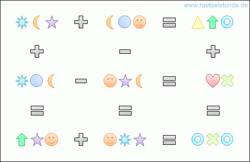
The program to solve is trivial:
    |solution|

    solution := Solver
	anySolutionFor:[
		|star8 moon star5 circle face
		 tria upArrow ring heart cross
		 n11 n12 n13 n21 n22 n23 n31 n32 n33|

		star8 := (0 %% 9) name:'star8'.
		moon := (0 %% 9) name:'moon'.
		star5 := (0 %% 9) name:'star5'.
		circle := (0 %% 9) name:'circle'.
		face := (0 %% 9) name:'face'.
		tria := (0 %% 9) name:'tria'.
		upArrow := (0 %% 9) name:'upArrow'.
		ring := (0 %% 9) name:'ring'.
		heart := (0 %% 9) name:'heart'.
		cross := (0 %% 9) name:'cross'.

		Solver allDistinct:{ star8 . moon . star5 . circle . face .
				     tria . upArrow . ring . heart . cross }.
		n11 := (star8*100) + (moon*10) + star5.
		n12 := (moon*100) + (circle*10) + face.
		n13 := (tria*100) + (upArrow*10) + ring.

		n21 := (star8*100) + (circle*10) + moon.
		n22 := (face*100) + (star5*10) + moon.
		n23 :=              (heart*10) + cross.

		n31 := (upArrow*100) + (star5*10) + face.
		n32 := (face*100) + (star8*10) + star5.
		n33 := (ring*100) + (cross*10) + ring.

		(n11 + n12) =: n13.
		(n21 - n22) =: n23.
		(n31 + n32) =: n33.

		(n11 + n21) =: n31.
		(n12 - n22) =: n32.
		(n13 + n23) =: n33.

	    ].
     Transcript showCR:solution.

Eight Numbers Puzzle

Here is another puzzle which combines some topology:

     The eight number puzzle asks you to label the nodes of a graph
     with the values 1 to 8 such that no two connected nodes have consecutive values:

	   1--2
	  /|\/|\
	 / |/\| \
	3--4--5--6
	\  |\/| /
	 \ |/\|/
	   7--8

the nodes are numbered top-to-bottom, left to right.
    |rslt values|

    rslt :=
	Solver
	    findVariables: (
		(1 to:8) collect:[:idx |
		    { ('node%1' bindWith:idx) .  (1 %% 8) }
		]
	    )
	    suchThat:[:nodes |
		|connected|

		connected :=
		    [:i1 :i2 |
			((nodes atIndex:i1) - (nodes atIndex:i2)) abs >: 1.
		    ].

		connected value:1 value:2.
		connected value:2 value:6.
		connected value:6 value:8.
		connected value:8 value:7.
		connected value:7 value:3.
		connected value:3 value:1.
		connected value:1 value:4.
		connected value:4 value:7.
		connected value:2 value:5.
		connected value:5 value:8.
		connected value:1 value:5.
		connected value:2 value:4.
		connected value:4 value:8.
		connected value:5 value:7.
		connected value:3 value:4.
		connected value:4 value:5.
		connected value:5 value:6.
	    ].

    values := rslt values.

    Transcript showCR:('   %1--%2' bindWithArguments:values).
    Transcript showCR:'  /|\/|\ '.
    Transcript showCR:' / |/\| \ '.
    Transcript showCR:('%3--%4--%5--%6' bindWithArguments:values).
    Transcript showCR:'\  |\/| / '.
    Transcript showCR:' \ |/\|/  '.
    Transcript showCR:('   %7--%8 ' bindWithArguments:values).

Eight Queens Puzzle

Another classic is the 8-Queens puzzle. The goal os to place 8 queens onto a chessboard, so they dont hit each other:
Two interesting variants are found here: first, the queens are represented as Point instances, with their coordinates being FD-variables. Second, and more interesting is that one of the constraints is defined as a smalltalk validation-block.
    |problem solution "n"|

    problem := [
	    |queens xCoords yCoords checkDiagonals|

	    queens := (1 to:8) collect:[:qNr |
			Point
			    x:(1 %% 8 name:('q%1x' bindWith:qNr))
			    y:(1 %% 8 name:('q%1y' bindWith:qNr))
		      ].

	    xCoords := queens collect:[:q | q x].
	    yCoords := queens collect:[:q | q y].

	    "/ no two queens are in the same row
	    Solver allDistinct:yCoords.

	    "/ no two queens are in the same col
	    Solver allDistinct:xCoords.

	    "/ no two queens share the same diagonal
	    checkDiagonals :=
		[
		    |diag1 diag2|

		    queens do:[:q1 |
			q1 x isGround ifTrue:[
			    q1 y isGround ifTrue:[
				diag1 := q1 x value - q1 y value.
				queens do:[:q2 |
				    q2 ~~ q1 ifTrue:[
					q1 x isGround ifTrue:[
					    q1 y isGround ifTrue:[
						diag2 := q2 x value - q2 y value.
						diag1 = diag2 ifTrue:[ ConstraintException raise ].
					    ]
					].
				    ].
				].
			    ].
			].
		    ].
		].

	    Solver all:xCoords conform:[:qx | checkDiagonals value].
	    Solver all:yCoords conform:[:qy | checkDiagonals value].
	].

    "/ n := Solver countSolutionsFor:problem.
    "/ Transcript show:'there are '; show:n; showCR:' solutions.'.

    solution := Solver anySolutionFor:problem.
    Transcript showCR:solution.

Magic Squares

The magic squares problem is to label a n by n square so that the sum of every row, column and diagonal are equal. A normal magic square contains the integers 1 to n2. This is a very old kind of puzzle - dating back to ancient chinese mathematics.
Here is an example:
8 1 6
3 5 7
4 9 2
    |N problem solution|

    N := 3.
    problem :=
	[
	    |board|

	    board := TwoDimensionalArray rows:N cols:N.
	    1 to:N do:[:row |
		1 to:N do:[:col |
		    board atRow:row col:col put:(FDInt min:1 max:N squared).
		]
	    ].
	    "/ each row distinct
	    1 to:N do:[:row |
		Solver allDistinct:(board rowAt:row).
	    ].
	    "/ each col distinct
	    1 to:N do:[:col |
		Solver allDistinct:(board colAt:col).
	    ].
	    "/ diagonals
	    Solver allDistinct:(board firstDiagonal).
	    Solver allDistinct:(board secondDiagonal).
	].

    Transcript
	show:('there are %1 solutions.'
	      bindWith:(Solver countSolutionsFor:problem)).

    solution := Solver anySolutionFor:problem.
    Transcript showCR:solution.

Copyright © 2002 Claus Gittinger, all rights reserved

<info@exept.de>

Doc $Revision: 1.13 $ $Date: 2016/07/11 09:24:05 $